The Modern Spirit Of Statistical Arbitrage
Introduction
In this article, I would like to introduce statistical arbitrage (statarb) the way I understand it, as a practitioner at the forefront of the dark arts of statistical arbitrage.
If you google “statistical arbitrage”, you get the following from Wikipedia:
In finance, statistical arbitrage is a class of short-term financial trading strategies that employ mean reversion models involving broadly diversified portfolios of securities held for short periods of time. These strategies are supported by substantial mathematical, computational, and trading platforms.
A little more googling and one shall find that the quintessential statistical arbitrage implementation is that of pairs-trading. However, neither the Wikipedia entry nor pairs trading is a complete representation of what statarb is. I would even argue that the Wikipedia entry represents a very dated view on what statarb can be.
My main gripe with these definitions of statarb is that they miss the crux of what statarb is about, and instead choose to focus on a very narrow definition of statarb - that of mean-reversion signals.
Hence, today my goal is to provide an updated look at the essence of statarb, from the vantage point of a practitioner. If implementation details are sparse or vague, know that it is on purpose, you may PM me for clarifications, and I will likely selectively reply.
Summary
Statistical arbitrage is a class of strategy where we have
A portfolio of signals that
assign weights to instruments based on the relative out-performance(under-performance) of instruments in a basket (when we say relative, it is to some central point of all other instruments)
for a specific space (returns, price, volume, flow, dividends, etc).
The basket is also constructed such that net factor exposures of that basket tend towards 0, and majority of returns of that basket should come from the idiosyncratic returns space
This is the most updated definition of statistical arbitrage that encompasses all possibilities. I also believe that this is the definition of statistical arbitrage that is implied when interviewing for roles in podshops.
A more explicit example is the following:
Suppose there exists a dataset that provides predicted flow data for 3 stocks, NVDA, AMD, and AAPL. Let’s say there is $100mm, $150mm and -$100mm of predicted flow for NVDA, AMD and AAPL respectively.
An index rebal PM will form a portfolio with weights equal to
index_rebal_signal = [
    100/(100+150+100),
    150/(100+150+100),
    -100/(100+150+100)
]
index_rebal_signal = [
   0.286,
   0.429,
   -0.286
]
And his rationale would be clear and intuitive, there is 100mm of flow for NVDA and AMD, so prices will be going up, and there’s -100mm of flow for AAPL, so prices will be going down. We can then form a signal weighted by the magnitude of the flow. He will then purchase a hedging basket to dollar or factor neutralize his exposures to remove any unintended bets.
A statarb PM will likely form a portfolio with weights equal to
statarb_signal = [
    100-((100+150-100)/3),
    150-((100+150-100)/3),
    -100-((100+150-100)/3)
]
statarb_signal = [
   w/np.sum(np.abs(statarb_signal )) for w in statarb_signal
]
statarb_signal = [
   0.167,
   0.333,
   -0.5
]
See, from the statarb PM’s vantage point, it doesn’t matter that there is 100mm magnitude of flow for both NVDA (100mm) and AAPL (-100mm). What matters is that relative to AMD (150mm), NVDA has less flow (100mm), so NVDA should have less weight than AMD.
And although the magnitude of AAPL (-100mm) is smaller than AMD, relative to a central point (the mean in this case), AAPL is much further in displacement and hence should have more relative (in magnitude) underperformance, and therefore should be assigned a larger weight.
If he believes this portfolio has no factor exposure, then the signal construction process ends here, otherwise, he will also construct a hedging basket such that the factor exposure of the signal has been nulled.
I am not making a statement about whether or not this method of thinking is optimal. Only that this is the de facto approach for signals in the statarb space.
Pairs Trading
How does pairs-trading fit into the modern definition? Is it wrong? Does it still hold?
Well, of course it does. It still represents a really good introduction to statarb, and one that we can use to build intuition onto more complex representations.
Mapping pairs-trading onto our updated definition, it is a specific form of a generalized cross-sectional returns reversion signal. It assigns weights based on the relative out-performance of an instrument’s displacement from the pair’s mean in the returns space.
generalized_cross_sectional_signal = returns.mean(axis-1) - returns
generalized_cross_sectional_signal = (
   generalized_cross_sectional_signal.divide(
      generalized_cross_sectional_signal.abs().sum(axis=1),
      axis=0
)
There are possibly hundreds of guides to pairs trading, so I will not bore readers with more material on pairs trading. I will only use exactly what I need, and explain nothing more. If you find yourself wanting for more information on pairs trading, please consult the Hudson and Thames Pairs Trading guide - the most comprehensive guide on the most outdated form of statistical arbitrage.
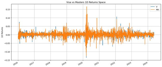
Pairs Trading: Visa And Masters Basket - Returns Space Signal
visa_masters_rets = visa_mastersclose.pct_change()
visa_masters_rets.plot(grid=True, figsize=(14, 6))
plt.title(’Visa vs Masters 1D Returns Space’)
plt.ylabel(’1D Returns’)
plt.show()
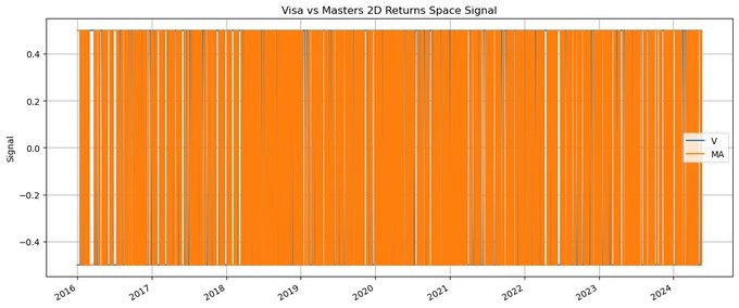
We can construct a signal following the principle described above. The raw signal is the displacement of the 2D returns of an instrument from the pair’s mean. If we (boldly) assume that visa and masters have similar factor loadings, we do not need to modify the existing weights, since being dollar neutral implies factor neutrality if the assumption holds.
visa_masters_rets_signal = -(
    visa_masters_rets.rolling(2).sum().subtract(
        visa_masters_rets.rolling(2).sum().mean(axis=1),
        axis=0
    )
)
visa_masters_rets_signal = (
    visa_masters_rets_signal.divide(
        visa_masters_rets_signal.abs().sum(axis=1),
        axis=0
    )
)

visa_masters_rets_signal.plot(grid=True, figsize=(14, 6))
plt.title(’Visa vs Masters 2D Returns Space Signal’)
plt.ylabel(’Signal’)
plt.show()
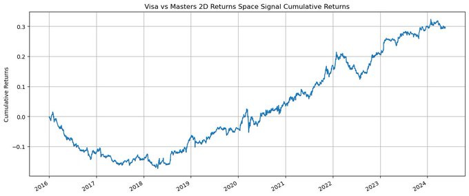
We can check how this signal would have done in the past.
visa_masters_rets_signal.shift(2).multiply(visa_masters_rets).sum(axis=1).cumsum().plot(grid=True, figsize=(14, 6))
plt.title(’Visa vs Masters 1D Returns Space Signal Cumulative Returns’)
plt.ylabel(’Cumulative Returns’)
plt.show()
Not too bad for a single pair. An annualized sharpe of 0.43, returns of 3.3%, and volatility of 7.5%; but this signal would not be tradeable on its own, as it has a high daily turnover of 36.8%.
Generalizing Pairs Trading: Banks Basket - Returns Space Signal
There is nothing magical about a pair. There were probably computational limitations 20 years ago that made only pairs viable as a statarb basket, and even traversing the search space of viable pairs was considered to be computationally intensive then.
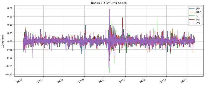
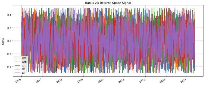
We can easily extend the same idea of betting on the relative displacement of the 2D returns of an instrument from the basket’s mean. We now turn to look at 5 banking stocks, JPM, BAC, C, MS, and GS.
We can extend the same signal to the 5 banking stocks, with the same assumptions.
banks_rets_signal = -(
    banks_rets.rolling(2).sum().subtract(
        banks_rets.rolling(2).sum().mean(axis=1),
        axis=0
    )
)
banks_rets_signal = (
    banks_rets_signal.divide(
        banks_rets_signal.abs().sum(axis=1),
        axis=0
    )
)

banks_rets_signal.plot(grid=True, figsize=(14, 6))
plt.title(’Banks 2D Returns Space Signal’)
plt.ylabel(’Signal’)
plt.show()
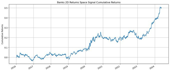
banks_rets_signal.shift(2).multiply(banks_rets).sum(axis=1).cumsum().plot(grid=True, figsize=(14, 6))
plt.title(’Banks 2D Returns Space Signal Cumulative Returns’)
plt.ylabel(’Cumulative Returns’)
plt.show()The signal has an annualized sharpe of 0.74, returns of 5.6%, and volatility of 7.5%, with a daily turnover of 19.5%.
Generalizing Banks Basket Into A Different Signal Space
Just like there is nothing special about the pair basket, there is nothing special about the returns space. We can easily generalize the signal into betting on the relative out-performance in another space.
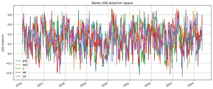
Suppose we have a hypothesis that instruments with higher autocorr in dollar volume will underperform as these instruments are getting an over-reaction that will correct.
We can then construct a signal in the dollar volume 20D auto-corr space.
banks_autocorr = banks.rolling(20).apply(lambda x: x.autocorr())

banks_autocorr.plot(grid=True, figsize=(14, 6))
plt.title(’Banks 20D AutoCorr Space’)
plt.ylabel(’20D AutoCorr’)
plt.show()
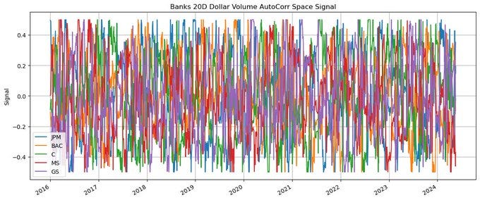
banks_autocorr_signal = -(
banks_autocorr.subtract(
banks_autocorr.mean(axis=1),
axis=0
)
)
banks_autocorr_signal = (
banks_autocorr_signal.divide(
banks_autocorr_signal.abs().sum(axis=1),
axis=0
)
)
banks_autocorr_signal.plot(grid=True, figsize=(14, 6))
plt.title(’Banks 20D AutoCorr Space Signal’)
plt.ylabel(’Signal’)
plt.show()banks_autocorr_signal.shift(2).multiply(banks_rets).sum(axis=1).cumsum().plot(grid=True, figsize=(14, 6))
plt.title(’Banks 20D AutoCorr Space Signal Cumulative Returns’)
plt.ylabel(’Cumulative Returns’)
plt.show()This signal is much more formidable than the other two, since it is in a space that is less contested than the 2D returns space, even for very large cap and well-known instruments.
The signal has an annualized sharpe of 1, returns of 6.1%, and volatility of 6.1%, with a daily turnover of 6.9%. This is probably a signal that can be traded on its standalone.
The State Of The Art
From my vantage point, the state-of-the-art of statistical arbitrage is the traversal of the search space for sensible baskets where “relative out-performance” makes sense, and for sensible spaces where relative outperformance in that space translates to relative outperformance in the idiosyncratic returns space.
The baskets are arbitrarily large, ranging from 2 instruments in the case of a pair, to 10000 instruments in the case of a global basket. Research is also being done on cross-asset baskets. The signal space is arbitrarily complex and can be constructed from multiple datasets.
Conclusion
Statistical arbitrage is about relative outperformance in any arbitrary sensible basket, in any arbitrary space, where a portfolio can be constructed such that factor returns are nullified and returns are majority idiosyncratic.


